SysID details

How the fit works and what it assumes: the procedure it follows, the 29 parameters it moves, the optimizer that moves them, and the excitations that make them observable. The steps to actually run it are in System identification.

Approach

We follow a procedure similar to OmniReset (UR5e), itself based on PACE (Bjelonic et al., 2025): record excitation runs on the real arm, replay them in sim under the same controller, and fit friction, armature and motor delay with CMA-ES to minimize the sim–real joint-trajectory error.

The one difference is the validation: the fitted parameters are scored on a run the optimizer never saw and that is not a chirp at all — the heldout multiband, recorded at stiffer gains than the fit. How the excitations are shaped, and why the chirp is split into two bands, is in Excitation design.

What is identified

29 parameters, all per joint except the last:

parameter	count	IsaacLab hook	bounds (default CLI)
armature (reflected rotor inertia)	7	write_joint_armature_to_sim	0 – 0.5 kg·m²
μ_static	7	write_joint_friction_coefficient_to_sim(static)	0 – 5 N·m
dynamic ratio (μ_dynamic = ratio · μ_static)	7	… (dynamic)	0 – 1
μ_viscous	7	… (viscous)	0 – 5 N·m·s/rad
motor delay	1	DelayedPDActuator lag buffers (pos/vel/effort)	0 – 4 ticks

Everything else — link masses/inertias, kinematics, the controller — is taken as known. Gravity is disabled on the sim articulation, mirroring libfranka’s gravity compensation on the real side.

The control law is indeed the same on both sides — τ = Jᵀ F, pure task-space PD (control_mode="task_impedance" in isaaclab_sysid/.../franka_sysid/control.py). The Jacobian in it is not obtained the same way:

• Real (src/osc_shm.cpp): libfranka’s analytic model, model.zeroJacobian(Frame::kEndEffector), about the EE frame configured in Desk — the same frame the pose is read from.

• Sim (franka_replay_env.py): PhysX body Jacobians from root_physx_view.get_jacobians(), averaged over panda_leftfinger and panda_rightfinger, while the pose and velocity are read from a third body, panda_fingertip_centered.

So J differs between the two in both its source and its reference point. CMA-ES absorbs that mismatch into the friction, armature and delay it fits — the identified parameters therefore carry some geometric error that does not belong to the joint dynamics at all.

Optimizer

The fit runs CMA-ES in isaaclab_sysid/scripts/tools/sysid_franka_osc.py, with the 29 parameters normalized to [0, 1] within the bounds above. Each generation evaluates --num_envs candidates on every run at once: each run gets its own block of --num_envs envs (the sim holds num_envs × runs envs), started from the run’s q_init and driven with the run’s gains from its sidecar, and env i of every block uses candidate i. The blocks replay on the same zero-order-hold time base as replay_python_csv_sim.py — a 50-tick warmup, then each 50 Hz setpoint held for its 20 × 1 ms ticks — and each candidate is scored at the CSV sample instants with

loss = w_q · MSE(q_sim − q_real) + w_dq · MSE(q̇_sim − q̇_real) + w_x · MSE(x_sim − x_real)
       (w_q = 1.0, w_dq = 0.1, w_x = 0.01 by default)

summed over trajectories with the weights of --traj_weights (default 1.0 each). The loss is a raw MSE, so a run counts in proportion to how far the arm moves in it; the high chirp band, which sweeps above the loop bandwidth and moves the arm far less than the low band, is nearly invisible next to it at equal weights. A fit on several runs prints what each run adds to the best candidate’s total (w*L of best): raise the weight of the run that stays behind and refit.

512 envs × 40 iterations take about 1 h on an RTX 5090; the cost of a 1 kHz tick barely depends on the env count, so a larger population is nearly free. The best parameters so far are saved every --save_interval generations to logs/sysid_franka/<timestamp>/checkpoint_<iter>.json, and the final result to logs/sysid_franka/<timestamp>/sysid_best_params.json.

--eval_params <file> skips the optimizer and rolls out one parameter set (a sysid_best_params.json or a checkpoint) on the given runs: it prints the loss per run and writes eval_rollout_<run>.csv and eval_result.json.

Excitation design

A parameter is identifiable only if the recorded motion exercises it. Two designs ship:

	multiband (python scripts/gen_excitation_traj.py / python examples/cart_impedance.py --mode multiband)	chirp (python scripts/gen_chirp_traj.py / python examples/cart_impedance.py --mode chirp)
Spectrum	three stationary tones per axis (0.15–0.30, 0.55–1.1 and 1.25–2.0 Hz), a tone at f having 0.35/f of the amplitude above 0.35 Hz	linear sweep on every axis, two bands: --band low 0.1 → 0.7 Hz at constant amplitude, --band high 0.7 → 3 Hz with the amplitude ∝ (0.7/f)^0.5
Active DOF	x, y, z, rx, ry (tilt about world x / y) + base-yaw	x, y, z, rx, ry, rz, π/3 phase-staggered
Amplitude (of the lowest tone)	6 / 6 / 6 cm; 0.20 / 0.15 rad of tilt, 0.25 rad of yaw	10 / 10 / 15 cm; 0.50 / 0.25 / 0.50 rad — the high band has these at 0.7 Hz and tapers to 48 / 48 / 72 mm; 242 / 121 / 242 mrad at 3 Hz
Envelope	2 s half-cosine fade-in and fade-out	linear: 2 s up / 3 s down (low band), 2 s up / 1 s down (high band)
Duration	12 s	8 s per band
Gains	kp 500 / 30 — the validation run	kp 200 / 20 — the low band is the fit run, the high band an optional held-out run (sized for these gains)

Design notes:

• Excite rotation. Translation alone barely moves j1 (base yaw) and j5 (wrist roll), leaving their friction unobservable. Adding yaw and roll to an earlier position-only excitation cut the sim–real RMS error from 88 to 39 mrad on j1 and from 29.5 to 10.1 mrad on j5.

• The wrist caps a constant-amplitude chirp at 0.7 Hz; the high band tapers instead. The single 0.1 → 3 Hz constant-amplitude sweep of the original UR5e / OmniReset design exceeds the 12 N·m limit of j5–j7 here and trips the tracking abort, so the low band stops at 0.7 Hz, where peak end-effector speed stays near 0.46 m/s. The high band continues to 3 Hz with the amplitude tapered as (0.7/f)^0.5 and a 1 s fade-out, so the upper third of the sweep runs at full envelope. It is sized for the fit gains kp 200/20, from an earlier run on the arm with taper exponent 1 and a 3 s fade-out:

  • The arm followed 0.44 / 0.20 / 0.11 of the z reference at 1.4 / 2.0 / 2.6 Hz. A 1-DOF model of the impedance loop (kd = 2√kp, 50 Hz zero-order hold) reproduces that roll-off with an effective mass of about 7.5 kg, i.e. a loop bandwidth √(kp/m)/2π of about 0.8 Hz at kp 200 (1.3 Hz at kp 500). The whole band lies above it: the motion falls as reference / f², and the load is set by the loop, not by the reference acceleration.

  • That left 34 / 11 / 2.8 mm of z motion around 2.5 / 4.5 / 6.5 s and 0.6–5 mrad per joint in the last window — too little to constrain anything, since the loss only scores motion — at a wrist load of 13 / 23 / 5 % of the limit (tau_J_limit_frac, gravity included).

  The model, calibrated on that run (z axis, kp 200; the first row is the run itself, measured 34 / 11 / 2.8 mm):

  taper exponent p, fade-out	reference at 3 Hz (z)	z motion around 2.5 / 4.5 / 6.5 s	peak force	torque step per 50 Hz setpoint
  1, 3 s (the run)	35 mm	43 / 11 / 3.3 mm	24 N	≈ 0.8 N·m
  0.5, 1 s (default)	72 mm	60 / 19 / 10 mm	33 N	≈ 1.6 N·m
  0, 1 s (constant amplitude, OmniReset)	150 mm	83 / 31 / 18 mm	44 N	≈ 3.1 N·m
  2, 3 s (constant reference acceleration)	8 mm	—	14 N	—

  The default’s motion and force are the model’s numbers; the run since made with it (kp 200/20, the chirp_high_fit run of the documented workflow) completed without an abort with the wrist at 14 / 27 / 5 % of its limit on j5–j7, where the model had put it near 30 %. The last column is why the default stops short of constant amplitude. Each 50 Hz setpoint is a step in commanded torque; osc_shm ramps any step above 0.8 N·m per tick (its 800 N·m/s slew limit), and the sim models neither that limit nor the 87 / 12 N·m clamp (it clamps at 100). At exponent 0 every setpoint would be followed by a ramp of about 4 ms that the sim does not have — the size of the whole 0–4 ms range the motor delay is searched in — and the fit would absorb it into delay and armature, the two parameters the high band is most sensitive to. At kp 500/30 the arm follows further up the band and the model puts the default at about 84 N: use --amp-taper-exp 2 there (about 30 N; the script warns).

• Replay at the logged rate. Targets are sent at 50 Hz and held by the 1 kHz controller; replay_python_csv_sim.py reproduces that hold, so the hold itself adds no sim–real mismatch. What does is the state in each 50 Hz row: it is the newest frame of the daemon’s 100 Hz stream, hence 0–10 ms older than the row’s nominal t_s — larger than the 0–4 ms motor delay the fit looks for. --log-1khz removes that: same setpoints at 50 Hz, but every controller tick recorded and each setpoint stamped by the tick it took effect (Data format). Never replay a 50 Hz log through a 1 kHz path.

• Hold the high band out. The fit sees the low band alone; the high band, the same design continued above the loop bandwidth, is an optional held-out run that checks how the identified armature and delay extrapolate — or a second fit run, if the identified dynamics should hold up better on high-acceleration motion.

• Validate on another waveform. A held-out chirp would share its waveform with the fit data: one frequency at a time, every axis at the same frequency. The heldout multiband puts all its tones in at once, a different frequency on every axis, over the same six DOFs and inside the fitted range (0.15–2 Hz against 0.1–3 Hz). Three choices make it a fair check of a chirp fit:

  • Tilt. Rotations about world x and y move the tool axis up to 20° off vertical, so j5 / j6 are exercised by commanded motion, not only by tracking error. Roll is off: with the tool pointing down it is the same rotation as yaw.

  • Spectrum. Tone amplitudes ∝ 0.35/f (constant peak reference velocity above the corner), so the upper two tones carry 12–33 % of the reference’s position power, depending on the axis — enough for the error on them to score armature, not friction alone.

  • Fade-out. It ends at the start pose.

  The profile has since run on the arm at kp 500/30, and is the held-out validation run behind Our results. It runs at those gains rather than the fit’s 200/20 because what limits its upper tones is the loop bandwidth measured above, not the reference.

Target trajectories

Multiband

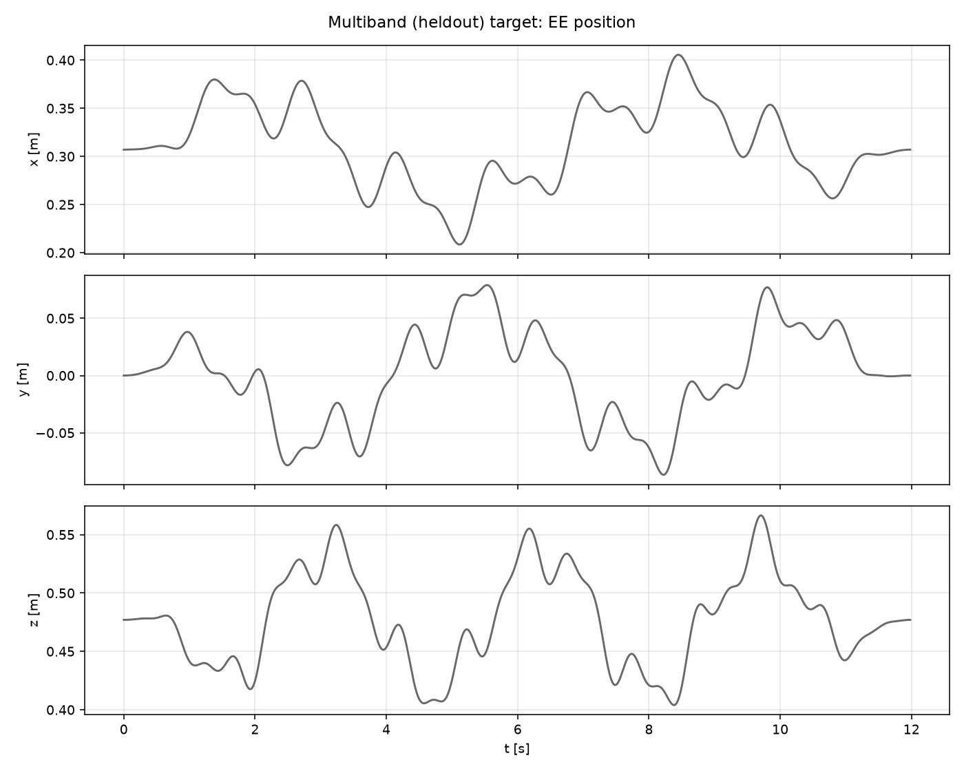
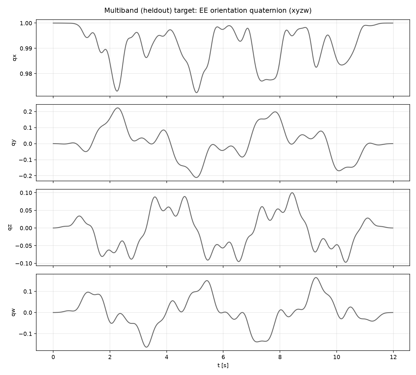
Three tones per axis under a 2 s half-cosine fade-in and fade-out, so the target starts and ends at the start pose. qz and qw move (±0.10 and ±0.16): they are the tilt about world x and y. The target orientation is yaw(t) about world z, applied after the tilt by the world-frame axis-angle vector (rx(t), ry(t), 0), applied to the start orientation.

Chirp, low band

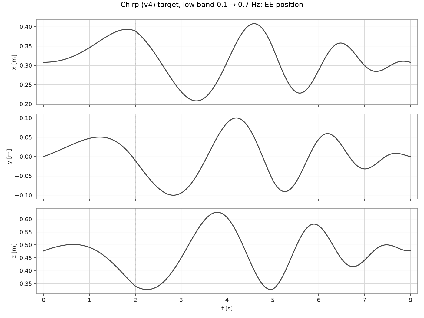
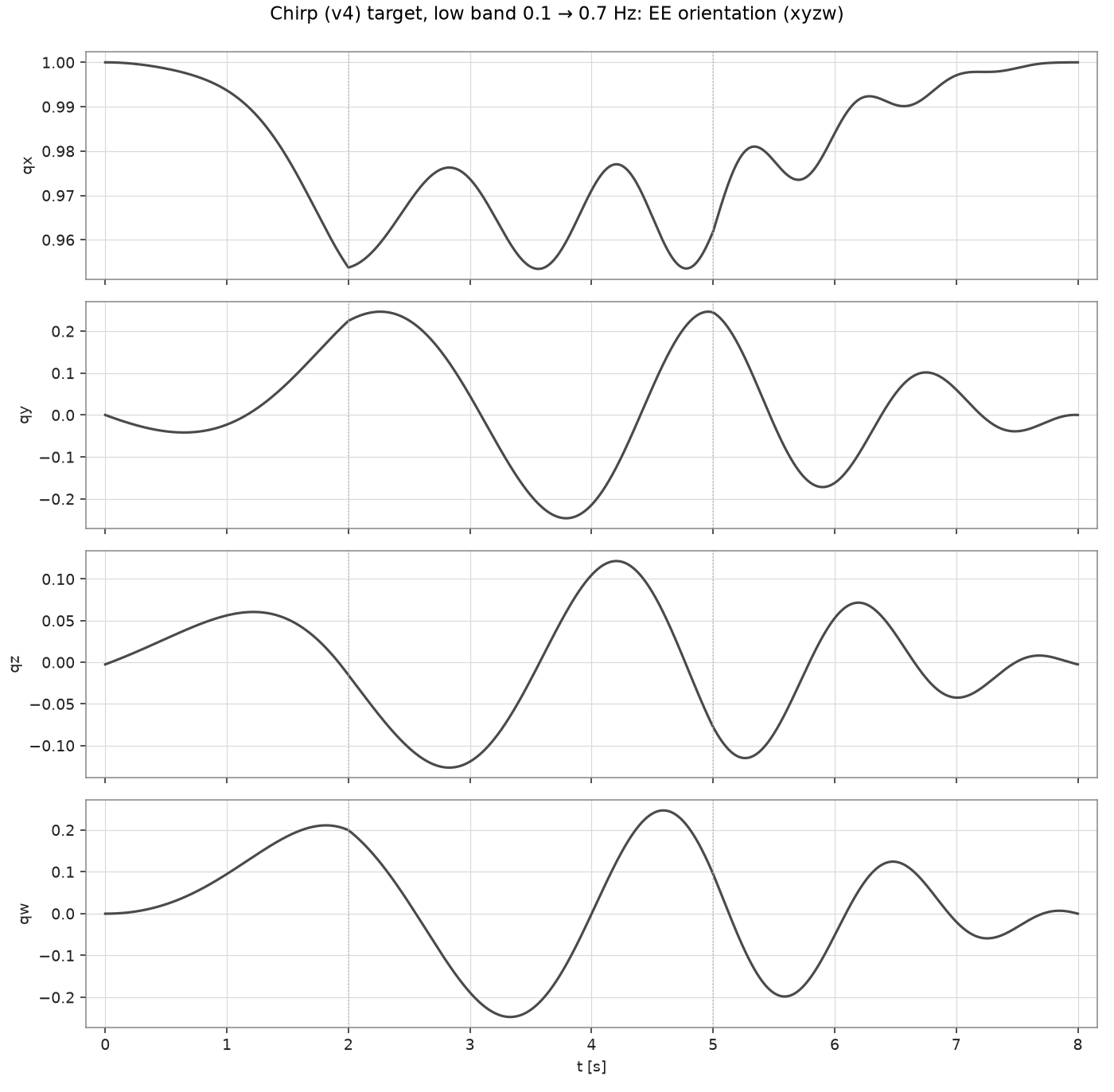
The envelope fades in over 2 s and out over 3 s, so the target ends at the start pose. The kinks at 2 s and 5 s are the corners of that linear envelope; since the fade-out coincides with the highest frequencies, the peak reference acceleration (1.3 m/s² on z) stays well below what the amplitudes would give at 0.7 Hz.

Chirp, high band

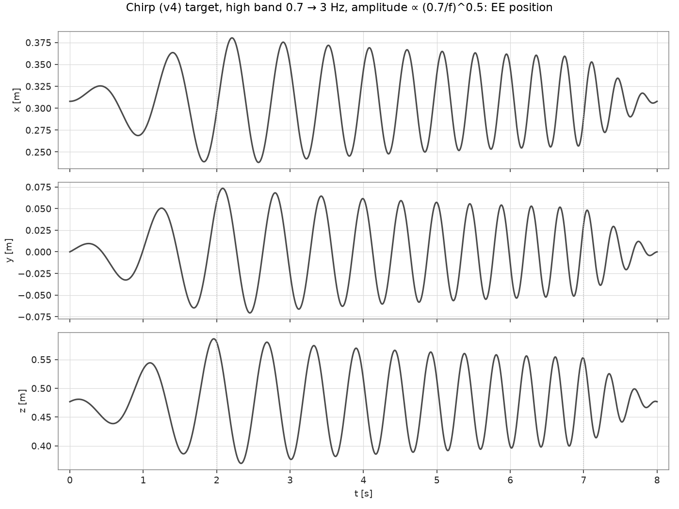
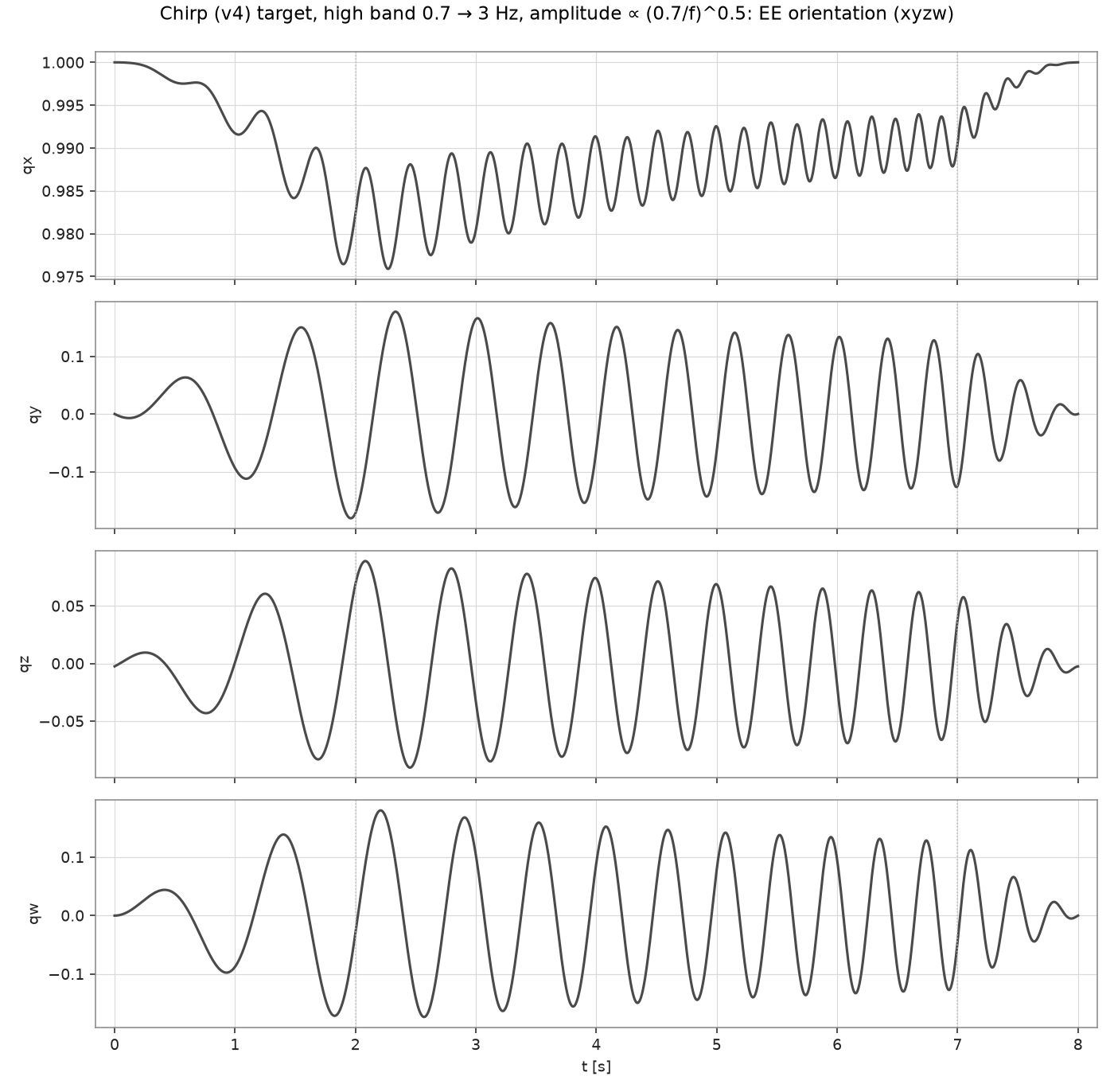
0.7 → 3 Hz with a 1 s fade-out, so the envelope stays at full amplitude from 2 s to 7 s. The (0.7/f)^0.5 taper shrinks the excursion as the sweep climbs — 11 cm on z at 2 s (1.3 Hz), 9 cm at 5 s (2.1 Hz), 7.5 cm at 7 s (2.7 Hz); the orientation stays within 0.44 rad of the anchor. The reference is much faster than the arm: above the loop’s bandwidth it follows only a fraction of it.